ACT-America CASA Ensemble

ACT-America: Ensembles of Biogenic C Fluxes for North America, 2003-2018

Download this document in PDF

Data Set Version: V1.1 (updated on July 12, 2019)

Note: In July 2019, the 2018 results were added and 2017 simulation were rerun with updated meteorological driver dataset.

Summary

This data set provides gridded, model-derived gross primary productivity (GPP), ecosystem respiration (RECO), and net ecosystem exchange (NEE) of CO₂ biogenic fluxes and their uncertainties at monthly and 3-hourly time scales over 2003-2018 on a 463-m resolution grid for the conterminous United States (CONUS) and also on a 5-km resolution grid for North America (NA). The 5-km results are further upscaled to a half-degree resolution. The biogeochemical model is Carnegie Ames Stanford Approach (CASA).

There are 708 files in NetCDF v4 format with this data set. This includes 420 files containing ensemble members of each carbon flux and 288 files that are the mean and standard deviation across ensemble members.

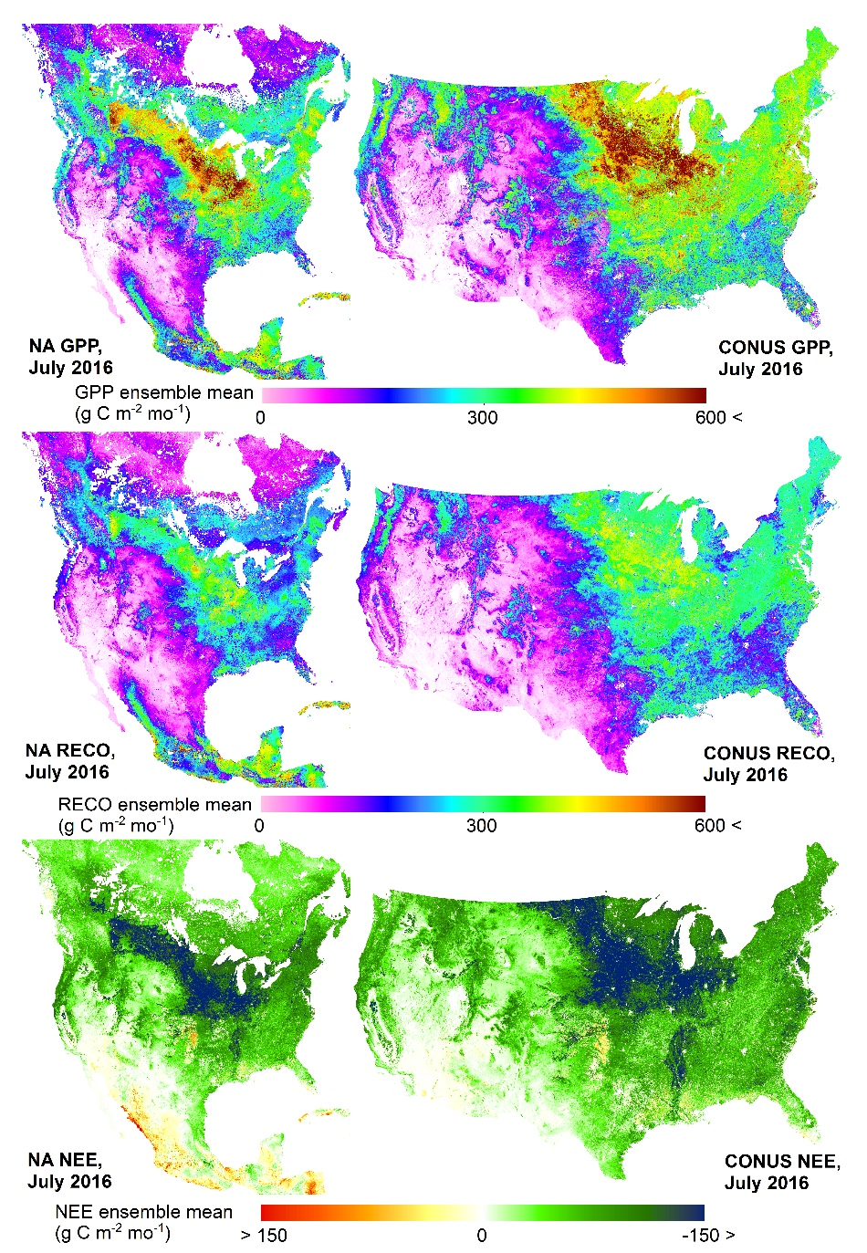
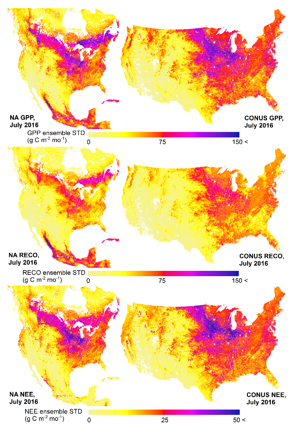
Figure 1. Mean and standard deviation of CASA L2 ensembles for three carbon fluxes (GPP, RECO, and NEE) and at 463-m resolution for the conterminous US (CONUS) and at 5-km resolution for North America (NA) in July of 2016.

 

Citation

Yu Zhou, Christopher A. Williams, Thomas Lauvaux, Sha Feng, Ian Baker, Yaxing Wei, Scott Denning, Klaus Keller, Kenneth J. Davis. ACT-America: Gridded Ensembles of Surface Biogenic Carbon Fluxes for North America and the Conterminous United States, 2003-2018. ORNL DAAC, Oak Ridge, Tennessee, USA. https://doi.org/10.3334/ORNLDAAC/1675.

 

Table of Contents

1. Data Set Overview

2. Data Characteristics

3. Application and Derivation

4. Quality Assessment

5. Data Acquisition, Materials, and Methods

6. Data Access

7. References

 

1. Data Set Overview

This dataset that contains the second-level (L2) ensemble member estimates of surface biogenic CO₂ exchanges between land and atmosphere across portions of North America, and including three carbon fluxes: gross primary productivity (GPP), ecosystem respiration (RECO), and net ecosystem exchange (NEE). Carbon flux ensembles are derived from Carnegie Ames Stanford Approach (CASA) biogeochemical model (Potter et al. 1993; Randerson et al. 1996) with 27 perturbed parameter sets. This product contains carbon fluxes for two spatial domains, the conterminous United States and North America and at two temporal scales, monthly and 3-hourly.

Project: Atmospheric Carbon and Transport (ACT-America)

The ACT-America, or Atmospheric Carbon and Transport - America, project is a NASA Earth Venture Suborbital-2 mission to study the transport and fluxes of atmospheric carbon dioxide and methane across three regions in the eastern United States. Each flight campaign will measure how weather systems transport these greenhouse gases. Ground-based measurements of greenhouse gases were also-collected. Better estimates of greenhouse gas sources and sinks are needed for climate management and for prediction of future climate.

 

2. Data Characteristics

Spatial Coverage: Conterminous United States and North America

Spatial Resolution: 463m, 5km, and half degree

Temporal Coverage: 2003-01-01 to 2018-12-31

Temporal Resolution: Monthly and 3-hourly (3-hourly data is available for North America domain in 2016-2018; other temporal and spatial spans can be generated at user’s end with provided R script)

Site boundaries: (All latitudes and longitudes are given in decimal degrees)

Site	Westernmost Longitude	Easternmost Longitude	Northernmost Latitude	Southernmost Latitude
CONUS	-130.1748	-60.5999	55.3236	20.0276
NA	-175.5350	-24.7704	70.3800	0.7843

 

Data Description:

There are 708 files in netCDF v4 format in this data set, including 420 files (204 monthly and 216 3-hourly files) containing ensemble members of each carbon flux and 288 files are the mean and standard deviation across ensemble members. CONUS (conterminous United States) files are at 463m×463m spatial resolution, NA (North America) files are at 5-km×5-km resolution, and NA_HalfDeg (upscaled North America) files are at half-degree resolution. The time dimension is defined as the middle time point of each time period (e.g., 15th day of Marches for monthly files; 1.5 hours of the first three-hour for 3-hourly files). Fill value and missing values are -9999 for all files.

Data file naming convention:

CASAensemble_CASA_LEVEL_Ensemble_TIMESCALE_Biogenic_CARBONFLUX_SPATIALDOMAIN_YEAR(MONTH).nc4

CASA_LEVEL_Ensemble_STATISTIC_TIMESCALE_Biogenic_CARBONFLUX_SPATIALDOMAIN_YEAR(MONTH).nc4

Where

CASALEVEL is the level of data product, we currently provide Level-2 (L2) and Level-2B (L2B).

TIMESCALE is either monthly or 3-hourly.

STATISTIC is the mean or standard deviation (STD) across ensemble members.

CARBONFLUX is GPP, RECO or NEE.

SPATIALDOMAIN is CONUS, NA, or NA_HalfDeg.

YEAR is the year of simulation.

MONTH is simulated month, which only used for 3-hourly data

Example file names:

CASA_L2B_Ensemble_Monthly_Biogenic_GPP_NA_2005.nc4

CASA_L2_Ensemble_Mean_Monthly_Biogenic_NEE_CONUS_2004.nc4

CASA_L2_Ensemble_3-Hourly_Biogenic_RECO_NA_201605.nc4

Spatial Reference Properties:

North America Data

Projection: Lambert Conformal Conic 2SP

Parameters:

projection units: meters

datum (spheroid): GCS_unnamed_ellipse (from NARR data)

            Semi major Axis: 6371200.0

Semi minor Axis: 6371200.0

Inverse Flattening: 0.0

1st standard parallel: 50 deg N

2nd standard parallel: 50 deg N

Central meridian: -107deg (W)

latitude of origin: 50 deg N

false easting: 0

false northing: 0

Upscaled North America Data

Projection: WGS 1984

Parameters:

Angular Unit: Degree (0.0174532925199433)

            Prime Meridian: Greenwich (0.0)

            Datum: D_WGS_1984

            Semi major Axis: 6378137.0

            Semi minor Axis: 6356752.314245179

            Inverse Flattening: 298.257223563

Conterminous United States Data

Projection: Lambert Conformal Conic

Parameters:

projection units: meters

datum (spheroid): GRS_1980

            Semi major Axis: 6378137.0

Semi minor Axis: 6356752.314140356

Inverse Flattening: 298.257222101

1st standard parallel: 50 deg N

2nd standard parallel: 50 deg N

Central meridian: -107deg (W)

Latitude of origin: 50 deg N

false easting: 0

false northing: 0

3-Hourly NARR files:

These files are examples of ancillary data from 3-hourly NARR data set (https://rda.ucar.edu/datasets/ds608.0/index.html#!description) to use the R script for temporal downscaling.

NARR_YEARMONTH_3h_FACTOR.tif

Where

YEAR is the year for temporal downscaling.

MONTH is selected month, which only used for 3-hourly data

FACTOR is either dwsw (downward shortwave radiation) or airt (air temperature at 2-m height).

 

3. Application and Derivation

Our product has finer spatial resolutions and a relatively long time span comparing to other available product. It could be used to access surface biogenic carbon fluxes across multiple spatial (hundred meters to continental) and temporal (hourly to annual) scales can give an indication of carbon cycle processes under different weather patterns and feedbacks to climate change.

Our ensemble product provides not only carbon flux estimates but also the uncertainty range. This data product also could serve as prior surface biogenic carbon fluxes for atmospheric inversion studies.

 

4. Quality Assessment

To test and confirm the accuracy of our monthly ensemble, the assessment was evaluated by a set of ground-truth data of measured carbon fluxes from the AmeriFlux database (sites are listed in Table 1) and other carbon flux products including 3-hourly MsTMIP modeled ensemble (Huntzinger et al. 2013; Fisher et al. 2016; Huntzinger et al. 2016), CarbonTracker 2017 (CT2017, Peters et al. 2007), SiB3 (Baker et al. 2008; Baker et al. 2013) from 2006 to 2010.

 

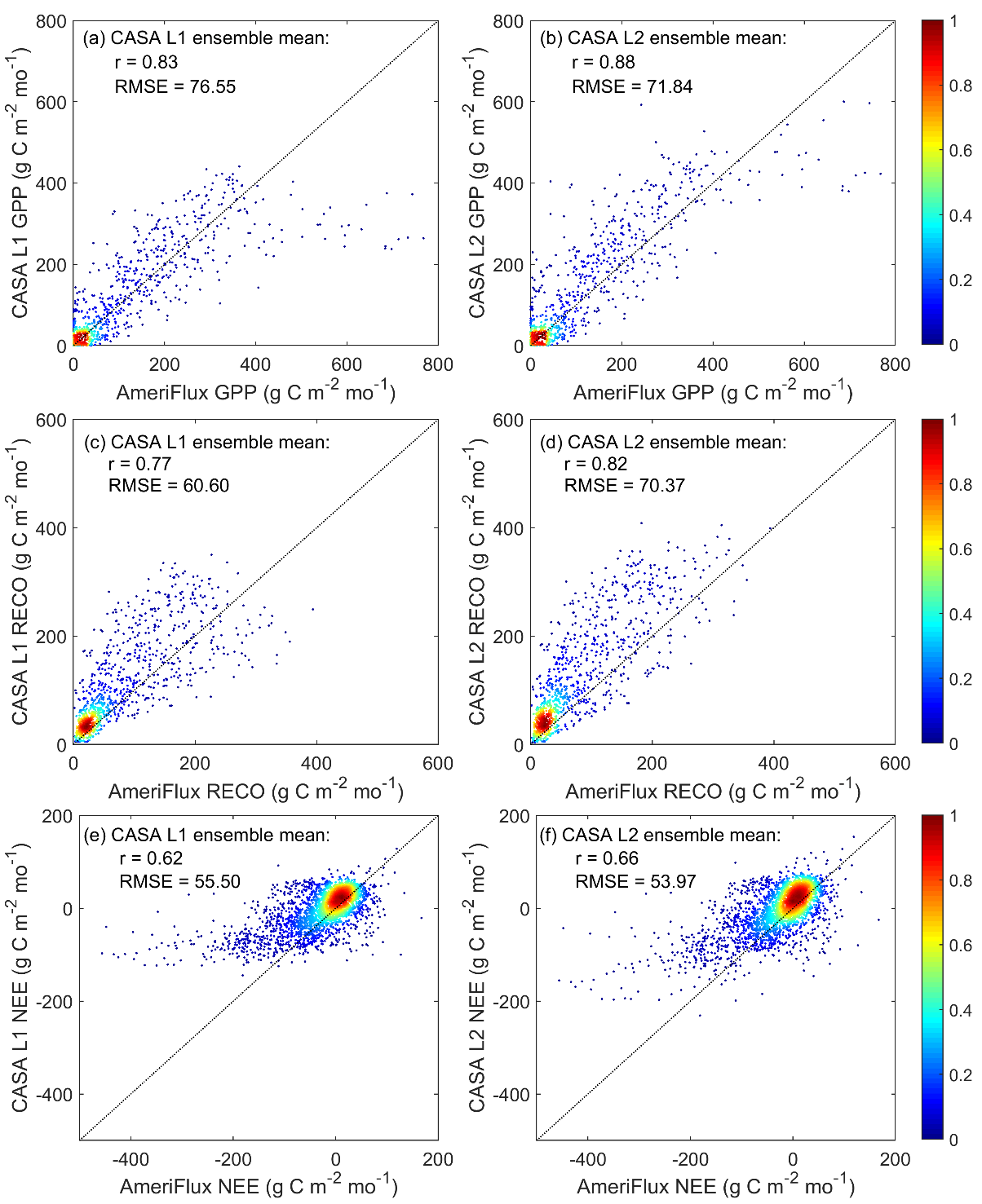
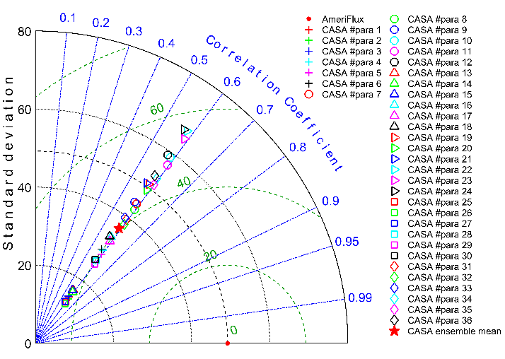
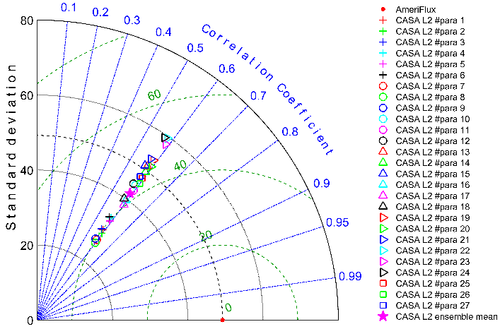
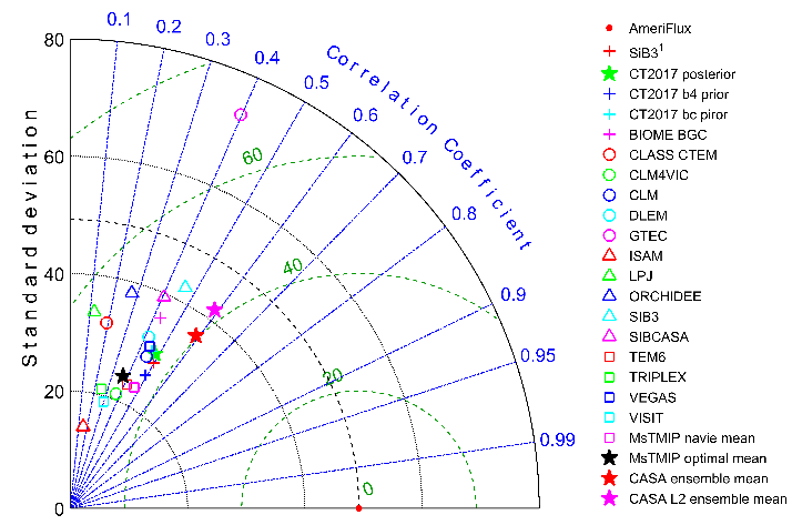
Table 1. List of AmeriFlux tower sites used in the quality assessment.

Site ID	Start Year	End Year	Lat	Lon	IGBP	Reference
US-AR1	2009	2012	36.4	-99.4	GRA	Billesbach et al. 2016a
US-AR2	2009	2012	36.6	-99.6	GRA	Billesbach et al. 2016b
US-ARb	2005	2006	35.5	-98.0	GRA	Torn 2006a
US-ARc	2005	2006	35.5	-98.0	GRA	Torn 2006b
US-ARM	2003	2012	36.6	-97.5	CRO	Fischer et al. 2007
US-Blo	1997	2007	38.9	-120.6	ENF	Goldstein et al. 2000
US-Cop	2001	2007	38.1	-109.4	GRA	Bowling 2007
US-EML	2008		63.9	-149.3	OSH	Belshe et al. 2012
US-GBT	1991	2006	41.4	-106.2	ENF	Massman 2006
US-GLE	2004	2014	41.4	-106.2	ENF	Frank et al. 2014
US-Goo	2002	2006	34.3	-89.9	GRA	Wilson and Meyers 2007
US-Ha1	1991	2012	42.5	-72.2	DBF	Urbanski et al. 2007
US-Ho2	1999		45.2	-68.7	ENF	Hollinger et al. 1999
US-Ho3	2000		45.2	-68.7	ENF	Hollinger et al. 1999
US-IB2	2004	2011	41.8	-88.2	GRA	Matamala 2018
US-KFS	2007		39.1	-95.2	GRA	Brunsell 2018a
US-Kon	2006		39.1	-96.6	GRA	Brunsell 2018b
US-KS2	2003	2006	28.6	-80.7	CSH	Powell et al. 2006
US-Lin	2009	2010	36.4	-119.8	CRO	Fares 2010
US-LPH	2002		42.5	-72.2	DBF	Hadley 2018
US-Me2	2002	2014	44.5	-121.6	ENF	Thomas et al. 2009
US-Me3	2004	2009	44.3	-121.6	ENF	Vickers et al. 2009
US-Me6	2010		44.3	-121.6	ENF	Ruehr et al. 2012
US-MMS	1999		39.3	-86.4	DBF	Schmid et al. 2000
US-Mpj	2007		34.4	-106.2	OSH	Litvak 2018a
US-MRf	2005		44.6	-123.6	ENF	Law 2018
US-Ne1	2001		41.2	-96.5	CRO	Verma et al. 2005
US-Ne2	2001		41.2	-96.5	CRO	Verma et al. 2005
US-Ne3	2001		41.2	-96.4	CRO	Verma et al. 2005
US-NR1	1998		40.0	-105.5	ENF	Monson et al. 2002
US-Oho	2004	2013	41.6	-83.8	DBF	Noormets et al. 2008
US-PFa	1995		45.9	-90.3	MF	Desai et al. 2015
US-Prr	2010	2014	65.1	-147.5	ENF	Nakai et al. 2013
US-Ro2	2003	2018	44.7	-93.1	CRO	Baker and Griffis 2017
US-SRC	2008	2014	31.9	-110.8	OSH	Kurc 2018
US-SRG	2008	2014	31.8	-110.8	GRA	Scott et al. 2015
US-SRM	2004	2014	31.8	-110.9	WSA	Scott et al. 2009
US-Sta	2005	2009	41.4	-106.8	OSH	Ewers and Pendall 2009
US-Syv	2001		46.2	-89.3	MF	Desai et al. 2005
US-Ton	2001		38.4	-121.0	WSA	Fischer et al. 2007
US-Twt	2009	2017	38.1	-121.7	CRO	Hatala et al. 2012
US-UMB	2000		45.6	-84.7	DBF	Gough et al. 2008
US-UMd	2007		45.6	-84.7	DBF	Gough et al. 2018
US-Var	2000		38.4	-121.0	GRA	Fischer et al. 2007
US-WCr	1999		45.8	-90.1	DBF	Cook et al. 2004
US-Whs	2007		31.7	-110.1	OSH	Scott et al. 2015
US-Wi1	2003	2003	46.7	-91.2	DBF	Chen 2003a
US-Wi2	2003	2003	46.7	-91.2	ENF	Chen 2003b
US-Wi3	2002	2004	46.6	-91.1	DBF	Chen 2005a
US-Wi5	2004	2004	46.7	-91.1	ENF	Chen 2004
US-Wi6	2002	2003	46.6	-91.3	OSH	Chen 2003c
US-Wi7	2005	2005	46.6	-91.1	OSH	Chen 2005a
US-Wi9	2004	2005	46.6	-91.1	ENF	Chen 2005b
US-Wjs	2007		34.4	-105.9	OSH	Litvak 2018b
US-Wkg	2004	2014	31.7	-109.9	GRA	Scott et al. 2010

 

5. Data Acquisition, Materials, and Methods

5.1 CASA description

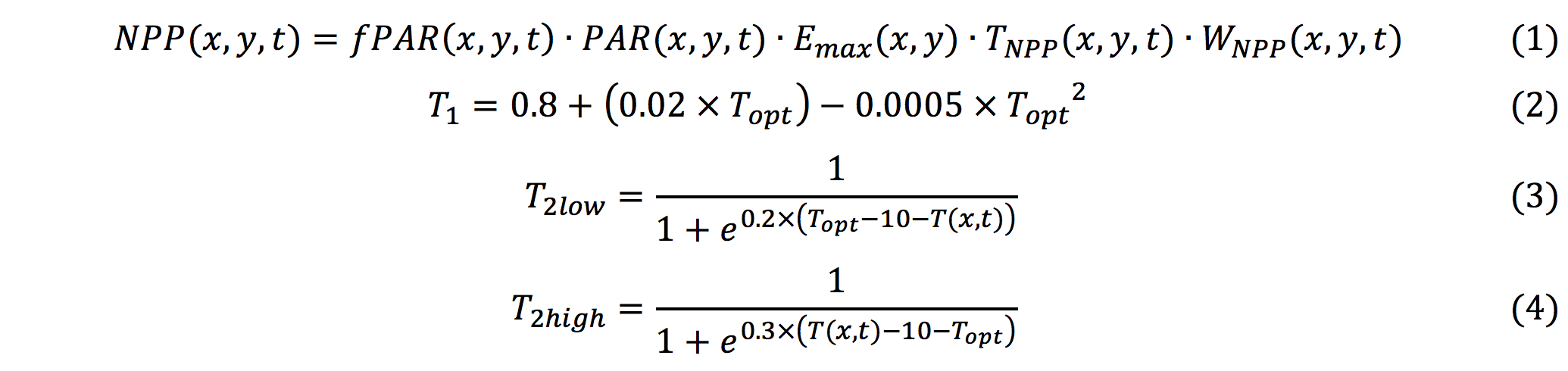
The modeling approach is based on the CASA biogeochemical model (Potter et al. 1993; Randerson et al. 1996). In CASA, NPP is calculated with a light use efficiency model driven by the absorbed fraction of photosynthetically active radiation (fPAR) and scaled by maximum light use efficiency (E_max), temperature scalar (T_NPP) and moisture stresses (W_NPP) at spatial location (x, y) and time (t) (Eq. 1). W_NPP is derived based on a ratio of estimated evapotranspiration to potential evapotranspiration, varying from 0.5 in arid ecosystem to 1 in very wet ecosystem. T_NPP is defined as T₁×T_2low×T_2high. T1 reflects the empirical observation that plants in very cold habitats typically have low maximum growth rate (Eq. 2). T₂ reflects the concept that the efficiency of light utilization should be depressed when plants are growing at temperatures displaces from their optimum (Eq. 3 and 4). T₂ has an asymmetric bell shape that falls off more quickly at high than at low temperatures. T_opt is defined as the air temperature in the month when the NDVI or LAI reaches its maximum for the year.

On a monthly time step, NPP is allocated to leaves, roots and wood (Eq. 5), with a default allocation ratio of 1:1:1. Each of these pools has a turnover time that specifies the rate at which carbon moves to litter pools (surface fine litter, soil fine litter, coarse woody debris). Carbon in the litterfall pool is either transferred to the microbial and soil organic matter pools or decomposed during the process (Fig. 1). Decomposition of dead pool (e.g. litter and soil organic pools) releases carbon, i.e. heterotrophic respiration (Rh), as Eq. 6:

where p is the number of pools, C_i is the carbon content of pool i, k_i is the pool-specific decay rate constant, W_resp and T_resp are the effect of soil moisture and temperature on decomposition, and D_ε is microbial carbon decomposition efficiency. The effect of temperature on soil carbon fluxes (T_resp) is treated uniformly as an exponential (Q10) response:

where Q₁₀ is the multiplicative increase in soil biological activity for a 10 ºC rise in soil temperature and T(x, t) is monthly averaged air temperature.

NEP is computed as:

We assumed a carbon use efficiency of 0.5 such that gross primary productivity (GPP) is 2×NPP. Correspondingly, total ecosystem respiration (RECO) would become the sum of NPP and Rh, and net ecosystem exchange (NEE) is equal to RECO – GPP. The data used as input to the model are listed in section 4.

For 3-hourly simulation, we used the North American Regional Reanlaysis (NARR) 3-hourly (UTC) air temperature (T_air) and downward shortwave radiation (DWSW) to further downscale monthly carbon fluxes. Here, we distributed monthly estimates to 3hourly temporal scale with a simple assumption of dependence on light for GPP and temperature for RECO (Olsen and Randerson 2004; Fisher et al. 2016).

where  is a temperature scalar, defined as following equation:

 

5.2 Full parameter sets for generating L1 data

Table 2. Perturbed parameter sets used to generate CASA ensemble Level-1 product.

#Para	1	2	3	4	5	6	7	8	9	10	11	12
ΔTopt	0	-2	2	0	-2	2	0	-2	2	0	-2	2
Emax	0.25	0.25	0.25	0.5	0.5	0.5	0.75	0.75	0.75	1	1	1
Q10	1.4	1.4	1.4	1.4	1.4	1.4	1.4	1.4	1.4	1.4	1.4	1.4
#Para	13	14	15	16	17	18	19	20	21	22	23	24
ΔTopt	0	-2	2	0	-2	2	0	-2	2	0	-2	2
Emax	0.25	0.25	0.25	0.5	0.5	0.5	0.75	0.75	0.75	1	1	1
Q10	1.2	1.2	1.2	1.2	1.2	1.2	1.2	1.2	1.2	1.2	1.2	1.2
#Para	25	26	27	28	29	30	31	32	33	34	35	36
ΔTopt	0	-2	2	0	-2	2	0	-2	2	0	-2	2
Emax	0.25	0.25	0.25	0.5	0.5	0.5	0.75	0.75	0.75	1	1	1
Q10	1.6	1.6	1.6	1.6	1.6	1.6	1.6	1.6	1.6	1.6	1.6	1.6
#Para	37	38	39	40	41	42	43	44	45	(Para 37 – 45 for cropland only)
ΔTopt	0	-2	2	0	-2	2	0	-2	2
Emax	1.25	1.25	1.25	1.25	1.25	1.25	1.25	1.25	1.25
Q10	1.4	1.4	1.4	1.2	1.2	1.2	1.6	1.6	1.6
Note: ΔTopt is the adjustment of optimal temperature.

 

5.3 Pruned parameter sets for generating L2 data

In order to further constrain E_max for each biome type, we use carbon flux measurements during the growing seasons from AmeriFlux and FLUXNET datasets (listed sites and corresponding years in Table S2) to infer the appropriate biome-specific range of E_max according to the light use efficiency model in CASA (Eq. 13). As flux sites are broadly distributed across space, we defined the growing season as months when the NPP is higher than averaged NPP within each year.

NPP_{obs_in} is the inferred NPP value from flux measurement, fPAR is derived from MOD15A2H at each flux site, and PAR_obs is the ground-measured at each site (for sites lacking PAR observation, we used NLDAS-2 instead). NPP scalars (T_NPP and W_NPP) are computed using ground-measured precipitation and air temperature (for sites lacking these observations, we used data sampled from PRISM at corresponding flux tower locations).

 

Table 3. Statistics of E_max inferred from flux tower data for each biome type to generate Level-2 data.

Biome type	WSA	CRO	DBF	ENF	MF	GRA	CSH	OSH
Grow Seas Avg	0.51	1.01	0.69	0.64	0.51	0.69	0.47	0.4
Grow Seas STD	0.04	0.37	0.15	0.23	0.29	0.29	0.29	0.15
Emax Samples for full Uncert. [E1, E2, E3]	[0.25, 0.50, 0.50]	[0.75, 1.00, 1.25]	[0.50, 0.75, 0.75]	[0.50, 0.75, 0.75]	[0.25, 0.50, 0.75]	[0.50, 0.75, 1.00]	[0.25, 0.50, 0.75]	[0.25, 0.50, 0.50]

 

Table 4. Perturbed parameter sets with constrained PFT-specific E_max used to generate CASA ensemble Level-2 product.

#Para	1	2	3	4	5	6	7	8	9
ΔTopt	0	-2	2	0	-2	2	0	-2	2
Emax	E1	E1	E1	E1	E1	E1	E1	E1	E1
Q10	1.4	1.4	1.4	1.2	1.2	1.2	1.6	1.6	1.6
#Para	10	11	12	13	14	15	16	17	18
ΔTopt	0	-2	2	0	-2	2	0	-2	2
Emax	E2	E2	E2	E2	E2	E2	E2	E2	E2
Q10	1.4	1.4	1.4	1.2	1.2	1.2	1.6	1.6	1.6
#Para	19	20	21	22	23	24	25	26	27
ΔTopt	0	-2	2	0	-2	2	0	-2	2
Emax	E3	E3	E3	E3	E3	E3	E3	E3	E3
Q10	1.4	1.4	1.4	1.2	1.2	1.2	1.6	1.6	1.6
Note: ΔTopt is the adjustment of optimal temperature.

 

5.4 Ecoregional sampling of Level-2 ensemble for generating Level-2B data

In addition to the Level-2 ensemble product, we added Level-2B to the data set which is the random sampling of Level-2 ensemble (27 members) based on the ecoregion maps. The Level-2B file, entitled with “CASA_L2B_Ensemble**”, has 10 members that randomly sampled L2 ensemble member (i.e., parameter set) for each Level-3 ecoregion for both North America and CONUS. Considering the data volume, we included only GPP and NEE for the Level-2B data. More information about ecoregion maps can be found at https://www.epa.gov/eco-research/ecoregions. Levels 1-3 ecoregion maps are available for North America; levels 1-4 ecoregion maps are available for conterminous US. The supplement contains an R script and converted ecoregion files (netcdf files) in order for users to generate the random sample for the ecoregion maps at other levels or change the number of samples.

5.5 Driver Data

Model input	Dataset	Spatial resolution	Time resolution	Reference
(a) Conterminous US
fPAR	MCD15A2H	463.31 m	8-day	Myneni et al. (2015)
Tree and herb covers	MOD44B	250 m	Yearly	Dimiceli et al. (2015)
Precipitation and Tair	PRISM	30 ″	Monthly	PRISM Climate Group (2016)
DWSW and DWLW1	NDLAS-2 Forcing	0.125 °	Monthly	LDAS (2016)
DWSW1 and Tair	NARR	32 km	3-hourly	NCEP (2005)
Biome type	National Forest Type	250 m	NA	Ruefenacht et al. (2008)
	NAFD	30 m	NA	Goward et al. (2012)
	MOD12Q1 IGBP	463.31 m	Yearly	Friedl et al. (2010)
Clay, silt, sand Fractions	CONUS-Soil	1000 m	NA	Miller and White (1998)
(b) North America
fPAR	MCD15A2	1000 m	8-day	Myneni et al. (2002)
Tree and herb covers	MOD44B	250 m	Yearly	Dimiceli et al. (2015)
Precipitation, Tair, DWSW, and DWLW1	NARR	32 km	Monthly	NCEP (2005)
DWSW and Tair	NARR	32 km	3-hourly	NCEP (2005)
Biome type	National Forest Type	250 m	NA	Ruefenacht et al. (2008)
	NAFD	30 m	NA	Goward et al. (2012)
	MOD12Q1 IGBP	463.31 m	Yearly	Friedl et al. (2010)
Clay, Silt, Sand Fractions	NACP MsTMIP Soil Map	0.25 °	NA	Liu et al. (2014)
1. DWSW and DWLW are downward shortwave and longwave radiation, respectively.

 

5.6 Guide of using R script for temporal downscaling

We provide the temporal downscaling codes written in R to enable users to estimate 3-hourly fluxes from monthly flux data. This script performs a temporal downscaling of monthly carbon flux estimates from a CASA model ensemble for two spatial domains, conterminous United States and North America. The R script uses three packages, including ncdf4, rgdal, and raster. One the users’ end,

1) users need to prepare the time series of 3-hourly NARR air temperature (in degree Celsius) and downward shortwave radiation for each month, separately, and change the path (NARRPath) in the script. We provide the 3-hoourly NARR examples for 2016-2018 with the R script;

2) users need to set the working dictionary to the path saved monthly ensemble (MonthlyEnsemblePath), and put the reference maps (NA_grid.tif and CONUS_grid.tif) into the working folder;

3) users can select the year (save3hrYear), month (save3hrMonth) and parameter set (save3hrParaSet, default is all 27 parameter sets) for temporal downscaling;

4) users can choose to save the 3-hourly outputs (Save3hrGPP, Save3hrRECO, Save3hrNEE).

Questions on how to prepare the 3-hourly NARR data or using this script can be forwarded to YuZhou2@clarku.edu (or CWilliams@clarku.edu)

 

5.7 Guide of using R script for random ecoregional sampling (Level-2B)

We provide a R script of random ecoregional sampling to generate the Level-2 ensemble at users’ end for two spatial domains, conterminous United States and North America. The R script uses three packages, including ncdf4, rgdal, and raster. On the users’ end,

1) users need to determine which ecoregional level to work with by define "EcoregionLevel". Levels 1-3 are available for North America; levels 1-4 are available for conterminous US. Here we have converted shapefiles of different levels from United States Environmental Protection Agency (https://www.epa.gov/eco-research/ecoregions) to the netcdf files that can be directly used in this script;

2) users need to define the spatial domain of the random ecoregional sampling: conterminous United States (CONUS) or North America (NA);

3) users need to set the path of ecoregion files (e.g., if users are working with level-3 ecoregions for conterminous United States, the ecoregion file is CONUS_Eco_Level3_CASAgrid.nc4);

4) users can define the number of Level-2B sampling by change "L2BMembers";

5) users need to set the path of Level-2 files by change "L2Path";

6) users can select the year(s) ("SampleYear") for sampling;

7) users can select the carbon flux(es) ("CFluxes") to be sampled;

8) If users would like to use the previous random samples for another sampling of a same spatial domain, please change "Saved_EcoregionRandSamp" to 1 and move the file "EcoregionRandSamp_**.txt" to the output path. This file should be found in the output path when "Saved_EcoregionRandSamp" is set to 0.

9) users can set the output path ("outputPath").

Questions on using this script can be forwarded to YuZhou2@clarku.edu (or cwilliams@clarku.edu)

 

6. Data Access

These data are available through the ACT-America Model Data Repository hosted at the Oak Ridge National Laboratory.

Data Access Link: ftp://evs2ftp.ornl.gov/Prior_Fluxes/Ecosystem_Fluxes/CASA_Ensemble/

Contact for Data Access Information:

E-mail: weiy@ornl.gov

For the L1 product, we perturbed the most sensitive parameters with the full 36 member suite of parameters (Table 3). This level of the product is not available online, please contact CWilliams@clarku.edu if you would like to use our L1 product.

 

Acknowledgement

This work was primarily funded by the Atmospheric Carbon and Transport (ACT) - America project, a NASA Earth Venture Suborbital 2 project supported by NASA’s Earth Science Division. Funding for this work came from the NASA ACT-America Project under award #NNX16AN17G and NNX15AG76G. This work used eddy covariance data acquired and shared by the FLUXNET community, including AmeriFlux and Fluxnet-Canada. Funding for AmeriFlux data resources was provided by the U.S. Department of Energy’s Office of Science. CarbonTracker (CT2017) results provided by NOAA ESRL, Boulder, Colorado, USA from the website at http://carbontracker.noaa.gov. Funding for the Multi-scale synthesis and Terrestrial Model Intercomparison Project (MsTMIP; https://nacp.ornl.gov/MsTMIP.shtml) activity was provided through NASA ROSES Grant #NNX10AG01A. Data management support for preparing, documenting, and distributing model driver and output data was performed by the Modeling and Synthesis Thematic Data Center at Oak Ridge National Laboratory (ORNL; http://nacp.ornl.gov), with funding through NASA ROSES Grant #NNH10AN68

 

7. References

Baker, I., Harper, A., da Rocha, H., Denning, A., Araújo, A., Borma, L., Freitas, H., Goulden, M., Manzi, A., & Miller, S. 2013. Surface ecophysiological behavior across vegetation and moisture gradients in tropical South America. Agricultural and Forest Meteorology, 182, 177-188

Baker, I., Prihodko, L., Denning, A., Goulden, M., Miller, S., & Da Rocha, H. 2008. Seasonal drought stress in the Amazon: Reconciling models and observations. Journal of Geophysical Research: Biogeosciences, 113

Baker, J., & Griffis, T. 2017. AmeriFlux US-Ro2 Rosemount- C7, doi:10.17190/AMF/1418683

Belshe, E., Schuur, E., Bolker, B., & Bracho, R. 2012. Incorporating spatial heterogeneity created by permafrost thaw into a landscape carbon estimate. Journal of Geophysical Research: Biogeosciences, 117

Billesbach, D., Bradford, J., & Torn, M. 2016a. AmeriFlux US-AR1 ARM USDA UNL OSU Woodward Switchgrass 1, doi:10.17190/AMF/1246137

Billesbach, D., Bradford, J., & Torn, M. 2016b. AmeriFlux US-AR2 ARM USDA UNL OSU Woodward Switchgrass 2, doi:10.17190/AMF/1246138

Bowling, D. 2007. AmeriFlux US-Cop Corral Pocket, doi:10.17190/AMF/1246129

Brunsell, N. 2018a. AmeriFlux US-KFS Kansas Field Station, doi:10.17190/AMF/1246132

Brunsell, N. 2018b. AmeriFlux US-Kon Konza Prairie LTER (KNZ), doi:10.17190/AMF/1246068

Chen, J. 2003a. AmeriFlux US-Wi1 Intermediate hardwood (IHW), doi:10.17190/AMF/1246015

Chen, J. 2003b. AmeriFlux US-Wi2 Intermediate red pine (IRP), doi:10.17190/AMF/1246017

Chen, J. 2003c. AmeriFlux US-Wi6 Pine barrens #1 (PB1), doi:10.17190/AMF/1246021

Chen, J. 2004. AmeriFlux US-Wi5 Mixed young jack pine (MYJP), doi:10.17190/AMF/1246020

Chen, J. 2005a. AmeriFlux US-Wi7 Red pine clearcut (RPCC), doi:10.17190/AMF/1246022

Chen, J. 2005b. AmeriFlux US-Wi9 Young Jack pine (YJP), doi:10.17190/AMF/1246024

Cook, B.D., Davis, K.J., Wang, W., Desai, A., Berger, B.W., Teclaw, R.M., Martin, J.G., Bolstad, P.V., Bakwin, P.S., & Yi, C. 2004. Carbon exchange and venting anomalies in an upland deciduous forest in northern Wisconsin, USA. Agricultural and Forest Meteorology, 126, 271-295

Desai, A.R., Bolstad, P.V., Cook, B.D., Davis, K.J., & Carey, E.V. 2005. Comparing net ecosystem exchange of carbon dioxide between an old-growth and mature forest in the upper Midwest, USA. Agricultural and Forest Meteorology, 128, 33-55

Desai, A.R., Xu, K., Tian, H., Weishampel, P., Thom, J., Baumann, D., Andrews, A.E., Cook, B.D., King, J.Y., & Kolka, R. 2015. Landscape-level terrestrial methane flux observed from a very tall tower. Agricultural and Forest Meteorology, 201, 61-75

Dimiceli, C., Carroll, M., Sohlberg, R., Kim, D.H., Kelly, M., & Townshend, J.R.G. 2015. MOD44B MODIS/Terra Vegetation Continuous Fields Yearly L3 Global 250m SIN Grid V006. NASA EOSDIS Land Processes DAAC. Available online: https://lpdaac.usgs.gov/dataset_discovery/modis/modis_products_table/mod44b_v006 (accessed on 26 July 2016)

Ewers, B., & Pendall, E. 2009. AmeriFlux US-Sta Saratoga, doi:10.17190/AMF/1246831

Fares, S. 2010. AmeriFlux US-Lin Lindcove Orange Orchard, doi:10.17190/AMF/1246830

Fischer, M.L., Billesbach, D.P., Berry, J.A., Riley, W.J., & Torn, M.S. 2007. Spatiotemporal variations in growing season exchanges of CO2, H2O, and sensible heat in agricultural fields of the Southern Great Plains. Earth interactions, 11, 1-21

Fisher, J.B., Sikka, M., Huntzinger, D.N., Schwalm, C., & Liu, J. 2016. 3-hourly temporal downscaling of monthly global terrestrial biosphere model net ecosystem exchange. Biogeosciences, 13, 4271-4277

Frank, J.M., Massman, W.J., Ewers, B.E., Huckaby, L.S., & Negrón, J.F. 2014. Ecosystem CO2/H2O fluxes are explained by hydraulically limited gas exchange during tree mortality from spruce bark beetles. Journal of Geophysical Research: Biogeosciences, 119, 1195-1215

Friedl, M.A., Sulla-Menashe, D., Tan, B., Schneider, A., Ramankutty, N., Sibley, A., & Huang, X. 2010. MODIS Collection 5 global land cover: Algorithm refinements and characterization of new datasets. Remote Sensing of Environment, 114, 168-182

Goldstein, A., Hultman, N., Fracheboud, J., Bauer, M., Panek, J., Xu, M., Qi, Y., Guenther, A., & Baugh, W. 2000. Effects of climate variability on the carbon dioxide, water, and sensible heat fluxes above a ponderosa pine plantation in the Sierra Nevada (CA). Agricultural and Forest Meteorology, 101, 113-129

Gough, C., Bohrer, G., & Curtis, P. 2018. AmeriFlux US-UMd UMBS Disturbance, doi:10.17190/AMF/1246134

Gough, C., Vogel, C., Schmid, H., Su, H.-B., & Curtis, P. 2008. Multi-year convergence of biometric and meteorological estimates of forest carbon storage. Agricultural and Forest Meteorology, 148, 158-170

Goward, S.N., Huang, C., Masek, J.G., Cohen, W.B., Moisen, G.G., & Schleeweis, K. 2012. NACP North American Forest Dynamics Project: Forest Disturbance and Regrowth Data. ORNL DAAC, Oak Ridge, Tennessee, USA. http://dx.doi.org/10.3334/ORNLDAAC/1077

Hadley, J. 2018. AmeriFlux US-LPH Little Prospect Hill, doi:10.17190/AMF/1246072

Hatala, J.A., Detto, M., Sonnentag, O., Deverel, S.J., Verfaillie, J., & Baldocchi, D.D. 2012. Greenhouse gas (CO2, CH4, H2O) fluxes from drained and flooded agricultural peatlands in the Sacramento-San Joaquin Delta. Agriculture, ecosystems & environment, 150, 1-18

Hollinger, D., Goltz, S., Davidson, E., Lee, J., Tu, K., & Valentine, H. 1999. Seasonal patterns and environmental control of carbon dioxide and water vapour exchange in an ecotonal boreal forest. Global Change Biology, 5, 891-902

Huntzinger, D., Schwalm, C., Michalak, A., Schaefer, K., King, A., Wei, Y., Jacobson, A., Liu, S., Cook, R., & Post, W. 2013. The north american carbon program multi-scale synthesis and terrestrial model intercomparison project–part 1: Overview and experimental design. Geoscientific Model Development, 6, 2121-2133

Huntzinger, D., Schwalm, C., Wei, Y., Cook, R., Michalak, A., Schaefer, K., Jacobson, A., Arain, M., Ciais, P., Fisher, J., Hayes, D.J., Huang, M., Huang, S., Ito, A., Jain, A.K., et al. 2016. NACP MsTMIP: Global 0.5-deg Terrestrial Biosphere Model Outputs (version 1) in Standard Format. ORNL DAAC, Oak Ridge, Tennessee, USA. https://doi.org/10.3334/ORNLDAAC/1225.

Kurc, S. 2018. AmeriFlux US-SRC Santa Rita Creosote, doi:10.17190/AMF/1246127

Law, B. 2018. AmeriFlux US-MRf Mary's River (Fir) site, doi:10.17190/AMF/1246049

LDAS 2016. NLDAS-2 Forcing Dataset, Land Data Assimilation Systems, at https://ldas.gsfc.nasa.gov/nldas/NLDAS2forcing.php (accessed on June 10, 2016)

Litvak, M. 2018a. AmeriFlux US-Mpj Mountainair Pinyon-Juniper Woodland, doi:10.17190/AMF/1246123

Litvak, M. 2018b. AmeriFlux US-Wjs Willard Juniper Savannah, doi:10.17190/AMF/1246120

Liu, S., Wei, Y., Post, W., Cook, R., Schaefer, K., & Thornton, M. 2014. NACP MsTMIP: Unified North American soil map. Available online: http://dx.doi.org/10.3334/ORNLDAAC/1242, Oak Ridge National Laboratory Distributed Active Archive Center, Oak Ridge, Tennessee, USA (accessed on 27 Jan 2017). In

Massman, B. 2006. AmeriFlux US-GBT GLEES Brooklyn Tower, doi:10.17190/AMF/1375200

Matamala, R. 2018. AmeriFlux US-IB2 Fermi National Accelerator Laboratory- Batavia (Prairie site), doi:10.17190/AMF/1246066

Miller, D.A., & White, R.A. 1998. A conterminous United States multilayer soil characteristics dataset for regional climate and hydrology modeling. [Available at http://EarthInteractions.org]. Earth interactions, 2, 1-26

Monson, R., Turnipseed, A., Sparks, J., Harley, P., Scott‐Denton, L., Sparks, K., & Huxman, T. 2002. Carbon sequestration in a high‐elevation, subalpine forest. Global Change Biology, 8, 459-478

Myneni, R., Knyazikhin, Y., & Park, T. 2015. MCD15A2H MODIS/Terra+Aqua Leaf Area Index/FPAR 8-day L4 Global 500m SIN Grid V006. NASA EOSDIS Land Processes DAAC. Available online: https://lpdaac.usgs.gov/dataset_discovery/modis/modis_products_table/mcd15a2h_v006 (accessed on 28 July 2016)

Myneni, R.B., Hoffman, S., Knyazikhin, Y., Privette, J., Glassy, J., Tian, Y., Wang, Y., Song, X., Zhang, Y., & Smith, G. 2002. Global products of vegetation leaf area and fraction absorbed PAR from year one of MODIS data. Remote Sensing of Environment, 83, 214-231

Nakai, T., Kim, Y., Busey, R.C., Suzuki, R., Nagai, S., Kobayashi, H., Park, H., Sugiura, K., & Ito, A. 2013. Characteristics of evapotranspiration from a permafrost black spruce forest in interior Alaska. Polar Science, 7, 136-148

NCEP, N.W.S.N.U.S.D.o.C. 2005. National Centers for Environmental Prediction (NCEP) North American Regional Reanalysis (NARR). In. Boulder, CO: Research Data Archive at the National Center for Atmospheric Research, Computational and Information Systems Laboratory

Noormets, A., McNulty, S.G., DeForest, J.L., Sun, G., Li, Q., & Chen, J. 2008. Drought during canopy development has lasting effect on annual carbon balance in a deciduous temperate forest. New Phytologist, 179, 818-828

Olsen, S.C., & Randerson, J.T. 2004. Differences between surface and column atmospheric CO2 and implications for carbon cycle research. Journal of Geophysical Research: Atmospheres, 109

Peters, W., Jacobson, A.R., Sweeney, C., Andrews, A.E., Conway, T.J., Masarie, K., Miller, J.B., Bruhwiler, L.M., Pétron, G., & Hirsch, A.I. 2007. An atmospheric perspective on North American carbon dioxide exchange: CarbonTracker. Proceedings of the National Academy of Sciences, 104, 18925-18930

Potter, C.S., Randerson, J.T., Field, C.B., Matson, P.A., Vitousek, P.M., Mooney, H.A., & Klooster, S.A. 1993. Terrestrial ecosystem production: a process model based on global satellite and surface data. Global Biogeochemical Cycles, 7, 811-841

Powell, T.L., Bracho, R., Li, J., Dore, S., Hinkle, C.R., & Drake, B.G. 2006. Environmental controls over net ecosystem carbon exchange of scrub oak in central Florida. Agricultural and Forest Meteorology, 141, 19-34

PRISM Climate Group 2016. PRISM Gridded Climate Data, Oregon State University, http://prism.oregonstate.edu (accessed on 20 July 2016). In

Randerson, J.T., Thompson, M.V., Malmstrom, C.M., Field, C.B., & Fung, I.Y. 1996. Substrate limitations for heterotrophs: Implications for models that estimate the seasonal cycle of atmospheric CO2. Global Biogeochemical Cycles, 10, 585-602

Ruefenacht, B., Finco, M., Nelson, M., Czaplewski, R., Helmer, E., Blackard, J., Holden, G., Lister, A., Salajanu, D., & Weyermann, D. 2008. Conterminous US and Alaska forest type mapping using forest inventory and analysis data. Photogrammetric Engineering & Remote Sensing, 74, 1379-1388

Ruehr, N.K., Martin, J.G., & Law, B.E. 2012. Effects of water availability on carbon and water exchange in a young ponderosa pine forest: Above-and belowground responses. Agricultural and Forest Meteorology, 164, 136-148

Schmid, H.P., Grimmond, C.S.B., Cropley, F., Offerle, B., & Su, H.-B. 2000. Measurements of CO2 and energy fluxes over a mixed hardwood forest in the mid-western United States. Agricultural and Forest Meteorology, 103, 357-374

Scott, R.L., Biederman, J.A., Hamerlynck, E.P., & Barron‐Gafford, G.A. 2015. The carbon balance pivot point of southwestern US semiarid ecosystems: Insights from the 21st century drought. Journal of Geophysical Research: Biogeosciences, 120, 2612-2624

Scott, R.L., Hamerlynck, E.P., Jenerette, G.D., Moran, M.S., & Barron‐Gafford, G.A. 2010. Carbon dioxide exchange in a semidesert grassland through drought‐induced vegetation change. Journal of Geophysical Research: Biogeosciences, 115

Scott, R.L., Jenerette, G.D., Potts, D.L., & Huxman, T.E. 2009. Effects of seasonal drought on net carbon dioxide exchange from a woody‐plant‐encroached semiarid grassland. Journal of Geophysical Research: Biogeosciences, 114

Thomas, C.K., Law, B.E., Irvine, J., Martin, J.G., Pettijohn, J.C., & Davis, K.J. 2009. Seasonal hydrology explains interannual and seasonal variation in carbon and water exchange in a semiarid mature ponderosa pine forest in central Oregon. Journal of Geophysical Research: Biogeosciences, 114

Torn, M. 2006a. AmeriFlux US-ARb ARM Southern Great Plains burn site- Lamont, doi:10.17190/AMF/1246025

Torn, M. 2006b. AmeriFlux US-ARc ARM Southern Great Plains control site- Lamont, doi:10.17190/AMF/1246026

Urbanski, S., Barford, C., Wofsy, S., Kucharik, C., Pyle, E., Budney, J., McKain, K., Fitzjarrald, D., Czikowsky, M., & Munger, J. 2007. Factors controlling CO2 exchange on timescales from hourly to decadal at Harvard Forest. Journal of Geophysical Research: Biogeosciences, 112

Verma, S.B., Dobermann, A., Cassman, K.G., Walters, D.T., Knops, J.M., Arkebauer, T.J., Suyker, A.E., Burba, G.G., Amos, B., & Yang, H. 2005. Annual carbon dioxide exchange in irrigated and rainfed maize-based agroecosystems. Agricultural and Forest Meteorology, 131, 77-96

Vickers, D., Thomas, C., & Law, B.E. 2009. Random and systematic CO2 flux sampling errors for tower measurements over forests in the convective boundary layer. Agricultural and Forest Meteorology, 149, 73-83

Wilson, T., & Meyers, T. 2007. Determining vegetation indices from solar and photosynthetically active radiation fluxes. Agricultural and Forest Meteorology, 144, 160-179